
XLOOKUP is one of the most powerful and user friendly functions in Excel. It replaces older lookup formulas and makes searching for data easier, safer, and more flexible.
If you have ever struggled with VLOOKUP errors or complex INDEX MATCH formulas, this guide will help. In this article, the XLOOKUP formula is explained step by step with clear examples so you can confidently use it in real spreadsheets.
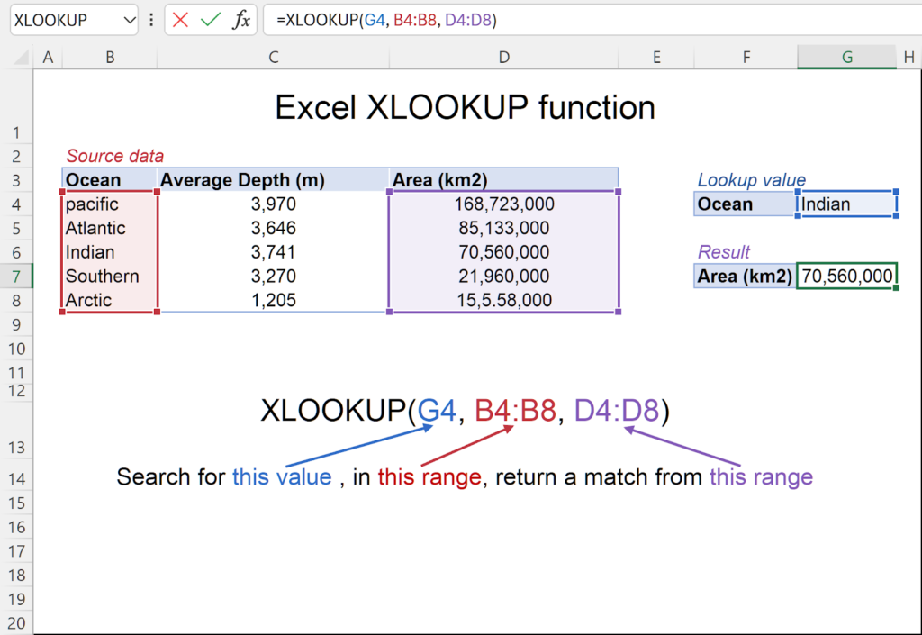
What Is the XLOOKUP Formula?
The XLOOKUP formula searches for a value in one range and returns a related value from another range.
It is commonly used to:
- Find names using IDs
- Return prices using product codes
- Match scores, dates, or categories
- Build clean and reliable reports
XLOOKUP works vertically and horizontally and returns exact matches by default.
XLOOKUP Formula Syntax Explained
The full XLOOKUP syntax looks like this:
=XLOOKUP(lookup_value, lookup_array, return_array, [if_not_found], [match_mode], [search_mode])
Here is what each part means:
- lookup_value is the value you want to find
- lookup_array is where Excel searches
- return_array is where Excel pulls the result from
- if_not_found defines what appears if no match exists
- match_mode controls exact or approximate matching
- search_mode controls the search direction
Most users only need the first three arguments.
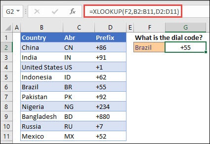
Example 1: Basic XLOOKUP Formula
Scenario:
- Column A contains product IDs
- Column B contains product names
You want to return the product name based on an ID entered in cell E2.
Formula:
=XLOOKUP(E2, A2:A20, B2:B20)
How it works:
- Excel searches A2:A20 for the value in E2
- When it finds a match, it returns the value from the same row in B2:B20

Example 2: XLOOKUP Searching to the Left
XLOOKUP can return values from columns on either side of the lookup column.
Scenario:
- Column B contains employee names
- Column A contains employee IDs
Formula:
=XLOOKUP(B2, B2:B20, A2:A20)
This searches column B and returns the matching ID from column A.
This is something VLOOKUP cannot do.
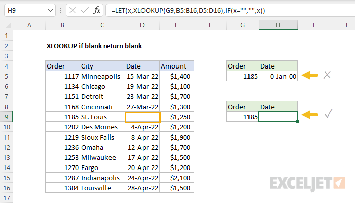
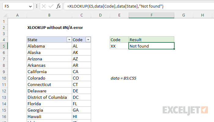
Example 3: Handling Missing Values
If XLOOKUP cannot find a value, it normally returns an error.
You can control this behavior using the if_not_found argument.
Formula:
=XLOOKUP(E2, A2:A20, B2:B20, “Not Found”)
Instead of an error, Excel displays a clear message.
Example 4: Horizontal XLOOKUP Formula
XLOOKUP works with rows as well as columns.
Scenario:
- Row 1 contains months
- Row 2 contains sales figures
Formula:
=XLOOKUP(B1, B1:F1, B2:F2)
This replaces the need for HLOOKUP.
Example 5: Returning Multiple Values with XLOOKUP
XLOOKUP can return multiple columns at once in modern Excel versions.
Formula:
=XLOOKUP(A2, A2:A10, B2:D10)
The result spills across cells automatically.
This is useful for dashboards and summary tables.
Example 6: Approximate Match Using XLOOKUP
XLOOKUP can return approximate matches for grading systems or pricing tiers.
Formula:
=XLOOKUP(E2, A2:A10, B2:B10,, -1)
This returns the closest smaller match.
Make sure lookup data is sorted correctly when using approximate matching.
Example 7: Finding the Last Match
XLOOKUP can search from bottom to top.
Formula:
=XLOOKUP(E2, A2:A20, B2:B20,, , -1)
This is useful for retrieving the most recent entry in a list.
Common XLOOKUP Formula Mistakes
Watch out for these issues:
- Lookup and return arrays with different sizes
- Including header rows accidentally
- Mixing text numbers with numeric values
- Using approximate match without sorting data
Most errors are fixed by checking range selection.
Why XLOOKUP Is Better Than Older Lookup Formulas
XLOOKUP improves on older functions by:
- Removing column index numbers
- Returning exact matches by default
- Allowing left and right lookups
- Including built in error handling
It replaces VLOOKUP, HLOOKUP, and LOOKUP in most situations.
Final Thoughts
Now that the XLOOKUP formula is explained with examples, you can start using it confidently in your spreadsheets.
XLOOKUP is flexible, powerful, and easy to maintain. Mastering it will save time and reduce errors in almost every Excel task.